Derivatives: Advanced Models

This notebook compares AbaQuant’s advanced option-pricing model family: Black–Scholes, Cox–Ross–Rubinstein (CRR) trees, Bachelier (normal volatility), Heston (stochastic volatility), Merton jump-diffusion, Normal-Inverse-Gaussian (NIG), SABR, and Variance-Gamma. It also covers model diagnostics, Monte Carlo/path simulation, and figures.

Assumption reminder: each advanced model relaxes a different Black–Scholes assumption (jumps, stochastic vol, heavy tails, …). Always check a model’s parameter constraints and limiting cases before comparing outputs across models — see docs/domains/assumptions.rst.

Sections:

1. Build one instance of each pricing model

2. Price all models

3. Model diagnostics

4. Simulations (Monte Carlo, GBM, Merton, Lévy)

5. Visualizations

Setup

import abaquant
print(f"AbaQuant version: {abaquant.__version__}")

AbaQuant version: 1.0.0rc1

import numpy as np

from abaquant.derivatives.analytics import distributions, parity, volatility
from abaquant.derivatives.models import (
    BlackScholesMertonModel,
    CoxRossRubinsteinModel,
    HestonStochasticVolatilityModel,
    MertonJumpDiffusionModel,
    NormalBachelierModel,
    NormalInverseGaussianModel,
    SABRVolatilityModel,
    VarianceGammaProcessModel,
)
from abaquant.derivatives.models.binomial import crr_tree_parameters
from abaquant.derivatives.models.black_scholes import bsm_d1_d2_summary
from abaquant.derivatives.models.merton import merton_jump_statistics
from abaquant.derivatives.monte_carlo import monte_carlo_bsm
from abaquant.derivatives.numerics.implied_volatility import implied_volatility_black_scholes
from abaquant.derivatives.simulation.gbm import simulate_gbm_paths
from abaquant.derivatives.simulation.levy import simulate_vg_nig_returns
from abaquant.derivatives.simulation.merton import simulate_merton_paths
from abaquant.visualization import VisualizationError

1. Build one instance of each pricing model

All models below share the same underlying spot (100), strike (100), and 1-year maturity so their outputs are directly comparable.

models = {
    "black_scholes": BlackScholesMertonModel(100.0, 100.0, 1.0, 0.05, 0.20),
    "crr": CoxRossRubinsteinModel(100.0, 100.0, 1.0, 0.05, 0.20, number_of_steps=50),
    "bachelier": NormalBachelierModel(100.0, 100.0, 1.0, 0.05, 20.0),
    "heston": HestonStochasticVolatilityModel(
        100.0, 100.0, 1.0, 0.05, 0.0, 0.04, 2.0, 0.04, 0.3, -0.5
    ),
    "merton": MertonJumpDiffusionModel(100.0, 100.0, 1.0, 0.05, 0.20, poisson_series_terms=8),
    "nig": NormalInverseGaussianModel(100.0, 100.0, 1.0, 0.05, 5.0, 0.0, 0.2),
    "sabr": SABRVolatilityModel(100.0, 100.0, 1.0, 0.20, 0.5, -0.3, 0.4),
    "variance_gamma": VarianceGammaProcessModel(100.0, 100.0, 1.0, 0.05, 0.20, -0.1, 0.2),
}
list(models.keys())

['black_scholes',
 'crr',
 'bachelier',
 'heston',
 'merton',
 'nig',
 'sabr',
 'variance_gamma']

2. Price all models

Call prices (or, for SABR, the ATM implied volatility) across the model family.

prices_by_model = {
    "black_scholes_call": models["black_scholes"].call_price(),
    "crr_put": models["crr"].put_price(),
    "bachelier_call": models["bachelier"].call_price(),
    "heston_call": models["heston"].call_price(),
    "merton_call": models["merton"].call_price(),
    "nig_call": models["nig"].call_price(),
    "sabr_implied_volatility": models["sabr"].implied_vol(),
    "variance_gamma_call": models["variance_gamma"].call_price(),
}
for name, value in prices_by_model.items():
    print(f"{name:26s}: {value:.6f}")

black_scholes_call        : 10.450584
crr_put                   : 5.533634
bachelier_call            : 10.276275
heston_call               : 10.368685
merton_call               : 13.288539
nig_call                  : 13.605323
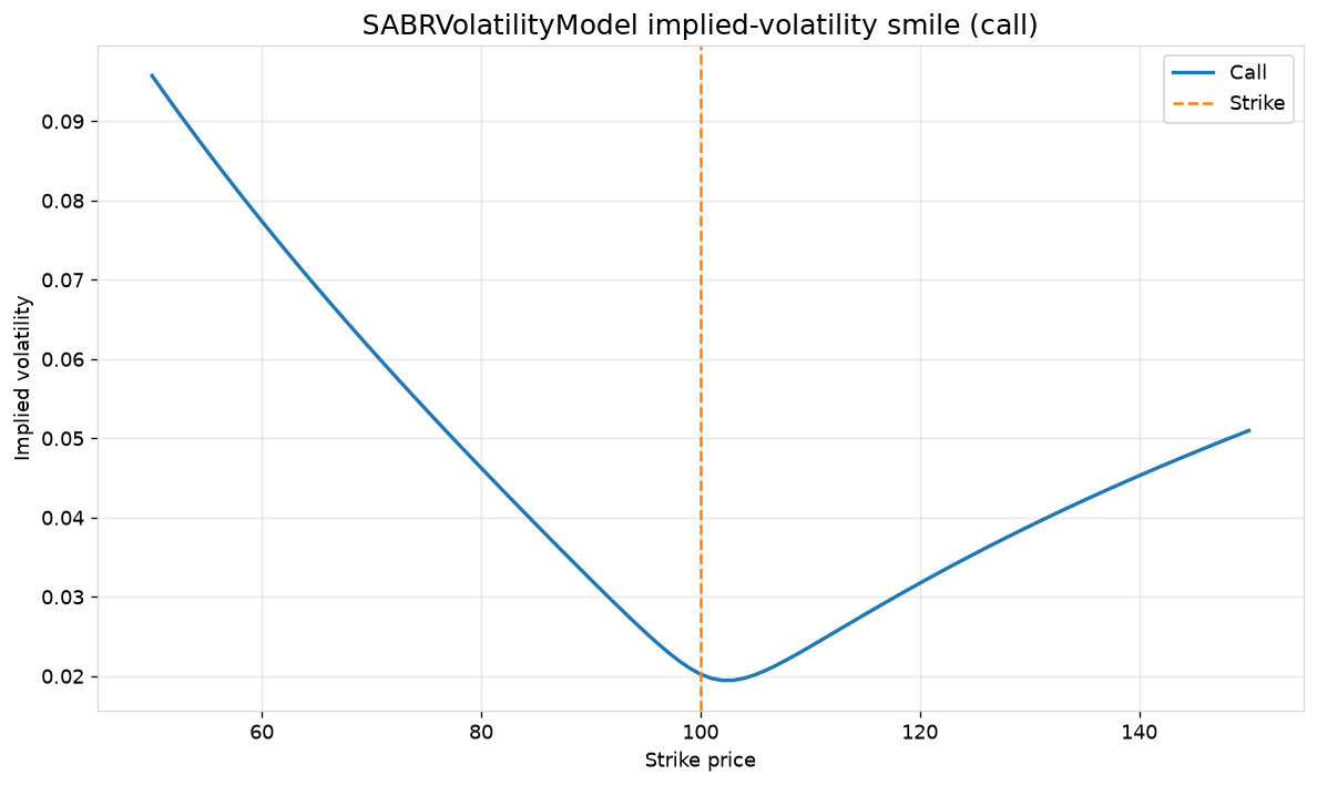
sabr_implied_volatility   : 0.020225
variance_gamma_call       : 11.266337

3. Model diagnostics

Analytical d1/d2 statistics, full scalar diagnostics reports, CRR tree parameters, Merton jump statistics, sample-distribution moments, a put-call-parity check, realized volatility, and a numerically solved implied volatility.

bsm_price = models["black_scholes"].call_price()
prices = np.array([100.0, 101.0, 99.0, 102.0, 103.0])

diagnostics = {
    "bsm_d1_d2": bsm_d1_d2_summary(100.0, 100.0, 1.0, 0.05, 0.20),
    "crr_tree_parameters": crr_tree_parameters(1.0, 0.05, 0.20, N=50),
    "merton_jump_statistics": merton_jump_statistics(1.0, -0.05, 0.20, 0.20),
    "distribution_moments": distributions.distribution_moments(prices),
    "parity_check": parity.parity_check(10.0, 7.0, 100.0, 100.0, 1.0, 0.05),
    "realized_volatility_last": float(volatility.realized_vol(prices, window=2)[-1]),
    "solved_bsm_iv": implied_volatility_black_scholes(bsm_price, 100.0, 100.0, 1.0, 0.05),
}
for key, value in diagnostics.items():
    print(f"{key}: {value}")

bsm_d1_d2: {'d1': 0.35000000000000003, 'd2': 0.15000000000000002}
crr_tree_parameters: {'dt': 0.02, 'u': 1.0286880693018583, 'd': 0.9721119840328972, 'p': 0.5106135568849628, 'disc': 0.999000499833375}
merton_jump_statistics: {'kappa_j': -0.029554466451491845, 'mean_jump_pct': -2.9554466451491845, 'lambda_adjusted': 0.9704455335485082, 'bsm_total_sigma': 0.28284271247461906}
distribution_moments: {'mean': 101.0, 'std': 1.4142135623730951, 'skew': 0.0, 'kurt': -1.3000000000000005}
parity_check: {'lhs': 3.0, 'rhs': np.float64(4.877057549928594), 'residual': np.float64(1.877057549928594)}
realized_volatility_last: 0.22558588810533645
solved_bsm_iv: 0.19999989181507927

call_diagnostics = models["black_scholes"].diagnostics("call").as_dict()
put_diagnostics = models["black_scholes"].diagnostics("put").as_dict()
call_diagnostics

{'option_type': 'call',
 'price': 10.450583572185565,
 'intrinsic_value': 0.0,
 'extrinsic_value': 10.450583572185565,
 'moneyness': 1.0,
 'forward_moneyness': 1.0512710963760241,
 'greeks': {'delta': 0.6368306511756191,
  'gamma': 0.018762017345846895,
  'vega': 0.3752403469169379,
  'theta': -0.01757267820941972,
  'rho': 0.5323248154537634,
  'vanna': -0.28143026018770345,
  'volga': 9.850059106569622,
  'charm': 0.00017990975537113463},
 'break_even_price': 110.45058357218556,
 'provenance': {'provider': 'derived',
  'dataset': 'derivative_diagnostics',
  'retrieved_at_utc': '2026-08-25T04:02:24+00:00',
  'cache_status': {},
  'source_labels': ['BlackScholesMertonModel', 'call'],
  'currency': None,
  'reporting_date': None,
  'transformation_steps': ['model pricing',
   'intrinsic value decomposition',
   'moneyness calculation',
   'Greek selection'],
  'request': {'model_class': 'BlackScholesMertonModel', 'option_type': 'call'},
  'notes': []}}

4. Simulations

Monte Carlo option pricing under Black–Scholes, plus raw path simulation under GBM, Merton jump-diffusion, and the Lévy-family (Variance-Gamma / NIG) return simulators.

simulations = {
    "monte_carlo_bsm": monte_carlo_bsm(100.0, 100.0, 1.0, 0.05, 0.20, n_paths=2_000),
    "gbm_shape": simulate_gbm_paths(100.0, 1.0, 0.05, 0.20, n_paths=8, n_steps=20)["paths"].shape,
    "merton_shape": simulate_merton_paths(100.0, 1.0, 0.05, 0.20, n_paths=8, n_steps=20)["paths"].shape,
    "levy_keys": sorted(
        simulate_vg_nig_returns(1.0, 0.20, -0.1, 0.2, 5.0, 0.0, 0.2, 0.2, n_sim=500).keys()
    ),
}
for key, value in simulations.items():
    print(f"{key}: {value}")

monte_carlo_bsm: {'price': 10.296010194210284, 'std_error': 0.12627131494649949, 'ci_95_lo': 10.048518416915146, 'ci_95_hi': 10.543501971505423, 'n_paths': 2000, 'bsm_price': 10.450583572185565, 'error_vs_bsm': 0.15457337797528048}
gbm_shape: (8, 21)
merton_shape: (8, 21)
levy_keys: ['gbm_returns', 'moments', 'nig_returns', 'vg_returns']

5. Visualizations

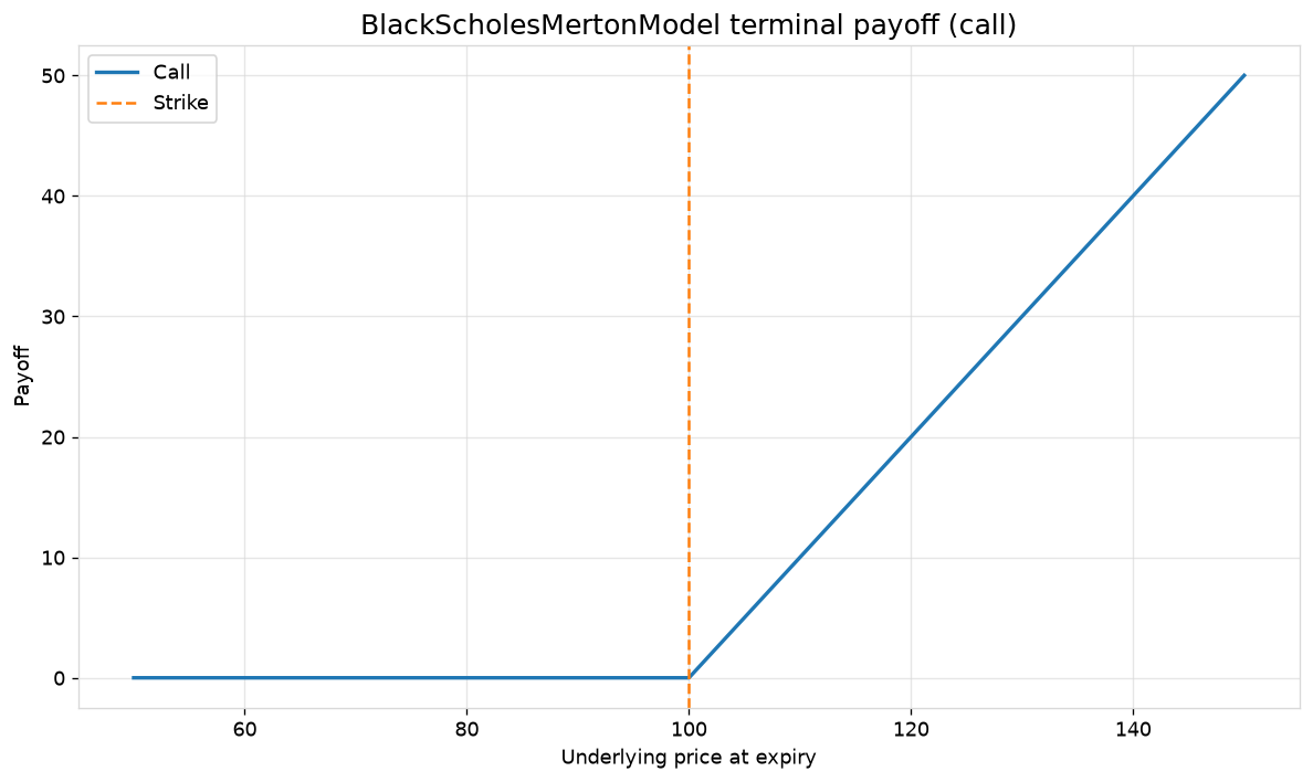
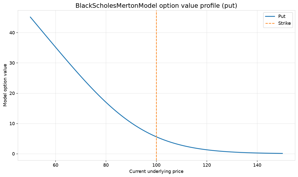
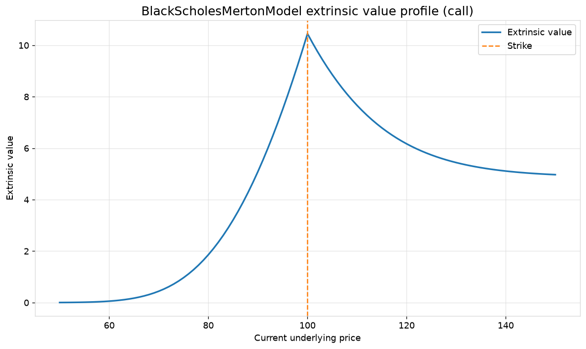
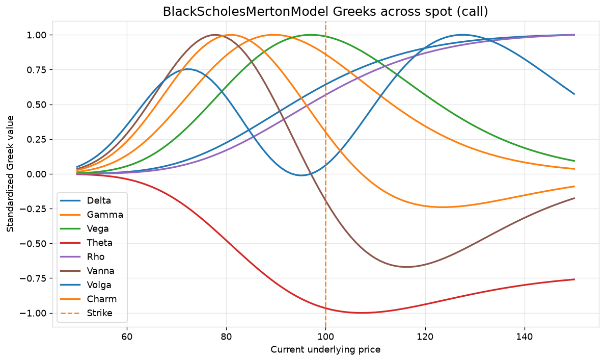
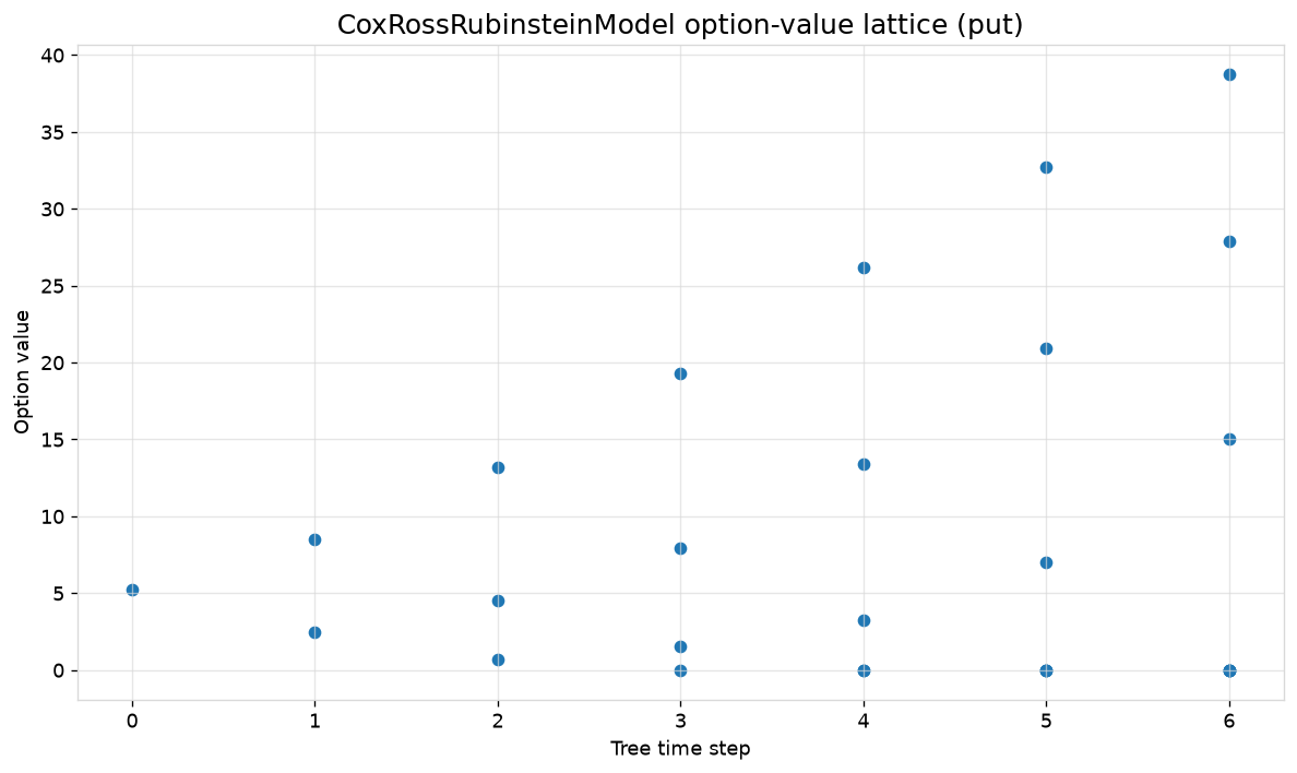
Payoff curves, price profiles, extrinsic value, standardized Greeks, price and delta surfaces, a CRR lattice, and the SABR volatility smile.

try:
    figures = {
        "bsm_call_payoff": models["black_scholes"].visualize(
            chart="payoff", option_type="call"
        ),
        "bsm_put_profile": models["black_scholes"].visualize(
            chart="price_profile", option_type="put"
        ),
        "bsm_call_extrinsic": models["black_scholes"].visualize(
            chart="extrinsic_value", option_type="call"
        ),
        "bsm_call_greeks": models["black_scholes"].visualize(
            chart="greeks", option_type="call", greek_scale="standardized"
        ),
        "crr_lattice": CoxRossRubinsteinModel(
            100.0, 100.0, 1.0, 0.05, 0.20, number_of_steps=6
        ).visualize(chart="tree", option_type="put"),
        "sabr_smile": models["sabr"].visualize(chart="volatility_smile"),
    }
    print(f"Created {len(figures)} figures: {list(figures)}")
except VisualizationError as exc:
    print(f"Visualization skipped (optional dependency missing): {exc}")

Created 6 figures: ['bsm_call_payoff', 'bsm_put_profile', 'bsm_call_extrinsic', 'bsm_call_greeks', 'crr_lattice', 'sabr_smile']

Takeaway

Each advanced model trades off tractability for extra realism (jumps, stochastic vol, heavy tails, negative rates). Use abaquant.derivatives.comparison.compare_all_models when you want a single call to price the same contract under several models side by side, and always sanity-check calibrated parameters — see the Assumptions and limitations guide in the docs.