Market Data (Offline)

This notebook demonstrates AbaQuant’s applied market-data facades — MarketTicker and MarketUniverse — using a deterministic, offline provider so the notebook runs without network access or a live data subscription. The same API works with a live provider (Yahoo, SEC, …) by simply swapping the provider= argument.

Sections:

1. A deterministic offline provider

2. Single-ticker workflow (quotes, options, financials)

3. Credit assessment from cached financials

4. Multi-ticker universe workflow

5. Visualizations

Setup

import abaquant
print(f"AbaQuant version: {abaquant.__version__}")

AbaQuant version: 1.0.0rc1

import pandas as pd

from abaquant.marketdata import get_ticker, get_tickers
from abaquant.visualization import VisualizationError

1. A deterministic offline provider

AbaQuant separates the facade (MarketTicker, MarketUniverse) from the provider that actually supplies data. Here we implement a small, self-contained provider returning fixed, repeatable values — the same pattern used throughout AbaQuant’s own test suite and examples.

def _sample_prices() -> pd.DataFrame:
    import numpy as np
    dates = pd.date_range("2025-01-02", periods=36, freq="B")
    trend = np.linspace(0.0, 1.0, len(dates))
    seasonal = np.sin(np.linspace(0.0, 4.0 * np.pi, len(dates)))
    return pd.DataFrame(
        {
            "ALPHA": 100.0 + 9.0 * trend + 1.8 * seasonal,
            "BETA": 82.0 + 6.0 * trend - 1.2 * seasonal,
            "GAMMA": 54.0 + 3.0 * trend + 0.7 * np.cos(np.linspace(0.0, 3.0 * np.pi, len(dates))),
        },
        index=dates,
    )


class DeterministicMarketDataProvider:
    """A repeatable, offline stand-in for a live market-data provider."""

    name = "deterministic-example"

    def fast_info(self, symbol: str) -> dict[str, float]:
        prices = _sample_prices()
        return {"lastPrice": float(prices.iloc[-1, 0])}

    def info(self, symbol: str) -> dict[str, object]:
        return {"currency": "USD", "marketCap": 600.0, "symbol": symbol}

    def history(self, symbol: str, **kwargs) -> pd.DataFrame:
        return pd.DataFrame({"Close": _sample_prices().iloc[:, 0]})

    def history_many(self, symbols, **kwargs) -> pd.DataFrame:
        return _sample_prices().reindex(columns=list(symbols))

    def option_expirations(self, symbol: str) -> list[str]:
        return ["2027-01-15", "2027-06-18", "2028-01-21"]

    def option_chain(self, symbol: str, expiry: str):
        shift = {"2027-01-15": 0.00, "2027-06-18": 0.025, "2028-01-21": 0.045}.get(expiry, 0.0)
        strikes = [80.0, 90.0, 100.0, 110.0, 120.0]
        calls = pd.DataFrame({
            "contractSymbol": [f"{symbol}C{int(k)}" for k in strikes],
            "strike": strikes,
            "lastPrice": [22.0, 14.5, 8.0, 4.5, 2.4],
            "bid": [21.5, 14.0, 7.6, 4.1, 2.0],
            "ask": [22.5, 15.0, 8.4, 4.9, 2.8],
            "impliedVolatility": [0.31 + shift, 0.27 + shift, 0.23 + shift, 0.25 + shift, 0.29 + shift],
            "openInterest": [120, 240, 520, 310, 180],
            "volume": [12, 28, 65, 34, 16],
        })
        puts = pd.DataFrame({
            "contractSymbol": [f"{symbol}P{int(k)}" for k in strikes],
            "strike": strikes,
            "lastPrice": [2.2, 4.1, 7.8, 13.9, 21.0],
            "bid": [1.9, 3.8, 7.4, 13.4, 20.4],
            "ask": [2.5, 4.4, 8.2, 14.4, 21.6],
            "impliedVolatility": [0.35 + shift, 0.30 + shift, 0.24 + shift, 0.26 + shift, 0.32 + shift],
            "openInterest": [210, 330, 610, 270, 155],
            "volume": [18, 36, 70, 29, 14],
        })
        return calls, puts

    def income_statement(self, symbol: str, *, period: str = "annual") -> pd.DataFrame:
        return pd.DataFrame({"2025-12-31": {
            "Total Revenue": 450.0, "EBITDA": 90.0, "EBIT": 75.0,
            "Interest Expense": 10.0, "Net Income": 60.0, "Gross Profit": 200.0,
        }})

    def balance_sheet(self, symbol: str, *, period: str = "annual") -> pd.DataFrame:
        return pd.DataFrame({"2025-12-31": {
            "Total Debt": 120.0, "Stockholders Equity": 300.0, "Current Assets": 250.0,
            "Inventory": 40.0, "Current Liabilities": 100.0, "Cash And Cash Equivalents": 50.0,
            "Total Assets": 500.0, "Total Liabilities": 200.0, "Retained Earnings": 110.0,
            "Long Term Debt": 80.0,
        }})

    def cash_flow_statement(self, symbol: str, *, period: str = "annual") -> pd.DataFrame:
        return pd.DataFrame({"2025-12-31": {"Operating Cash Flow": 70.0}})

2. Single-ticker workflow

Create one MarketTicker, then call quote, history, options, and financial-statement methods. Notice construction is lazy — no data is retrieved until you call a method.

provider = DeterministicMarketDataProvider()
ticker = get_ticker("DEMO", provider=provider, financial_cache="memory")

option_value = ticker.options.bsm(
    strike=100.0, maturity=0.5, risk_free_rate=0.04, volatility=0.20, option_type="call"
)
greeks = ticker.options.greeks(
    strike=100.0, maturity=0.5, risk_free_rate=0.04, volatility=0.20, option_type="call"
)
chain_analytics = ticker.options.analytics("2027-01-15")
iv_smile = chain_analytics.iv_smile(option_type="call")
rich_cheap = chain_analytics.rich_cheap_table(risk_free_rate=0.04, option_type="call")

print(f"Symbol:                    {ticker.symbol}")
print(f"Spot:                      {ticker.spot()}")
print(f"History rows (1mo):        {len(ticker.history.prices(period='1mo'))}")
print(f"Listed expirations:        {ticker.options.expirations()}")
print(f"BSM call value:            {option_value:.4f}")
print(f"Delta:                     {greeks['delta']:.4f}")
print(f"IV smile rows:             {len(iv_smile)}")
print(f"Largest rich-strike:       {float(rich_cheap.iloc[0]['strike'])}")
print(f"Total debt:                {ticker.financials.total_debt()}")
print(f"EBITDA:                    {ticker.financials.ebitda()}")

Symbol:                    DEMO
Spot:                      109.0
History rows (1mo):        36
Listed expirations:        ['2027-01-15', '2027-06-18', '2028-01-21']
BSM call value:            12.8921
Delta:                     0.7943
IV smile rows:             5
Largest rich-strike:       120.0
Total debt:                120.0
EBITDA:                    90.0

3. Credit assessment from cached financials

ticker.financials.credit_inputs() maps the cached statement snapshot into grouped CreditAnalysisInputs, which then feed into ticker.credit.assess(...). assess_from_financials() is a convenience wrapper that does both steps in one call.

inputs = ticker.financials.credit_inputs()
assessment = ticker.credit.assess(inputs)
from_financials = ticker.credit.assess_from_financials()

print(f"Input currency:       {inputs.reporting_currency}")
print(f"Synthetic score:      {assessment.synthetic_credit_proxy_score}")
print(f"Synthetic band:       {assessment.synthetic_credit_proxy_band}")
print(f"Convenience score:    {from_financials.synthetic_credit_proxy_score}")

Input currency:       None
Synthetic score:      96.34
Synthetic band:       strong_balance_sheet_proxy
Convenience score:    96.34

4. Multi-ticker universe workflow

MarketUniverse aligns multiple tickers behind one facade, exposing price/return panels, per-asset statistics, and portfolio construction.

universe = get_tickers(["ALPHA", "BETA", "GAMMA"], provider=provider)

prices = universe.history.prices(period="1mo")
returns = universe.history.returns(period="1mo")
stats_summary = universe.statistics.summary(period="1mo")
portfolio = universe.portfolio.max_sharpe(period="1mo", risk_free_rate=0.02)

print(f"Symbols:              {universe.symbols}")
print(f"Price panel shape:    {prices.shape}")
print(f"Return panel shape:   {returns.shape}")
print(f"Statistics rows:      {len(stats_summary)}")
print(f"Max-Sharpe first wt:  {float(next(iter(portfolio.weights.values()))):.4f}")
print(f"Max-Sharpe ratio:     {portfolio.sharpe_ratio:.4f}")

Symbols:              ('ALPHA', 'BETA', 'GAMMA')
Price panel shape:    (36, 3)
Return panel shape:   (35, 3)
Statistics rows:      3
Max-Sharpe first wt:  0.4500
Max-Sharpe ratio:     626.4701

5. Visualizations

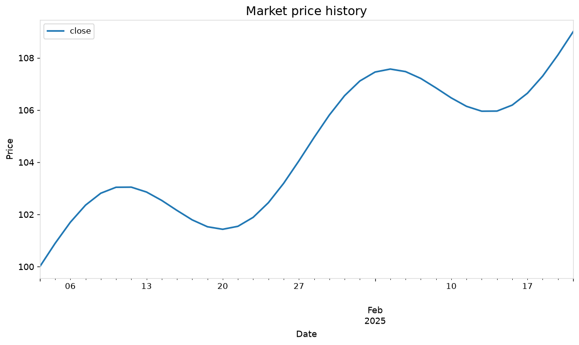
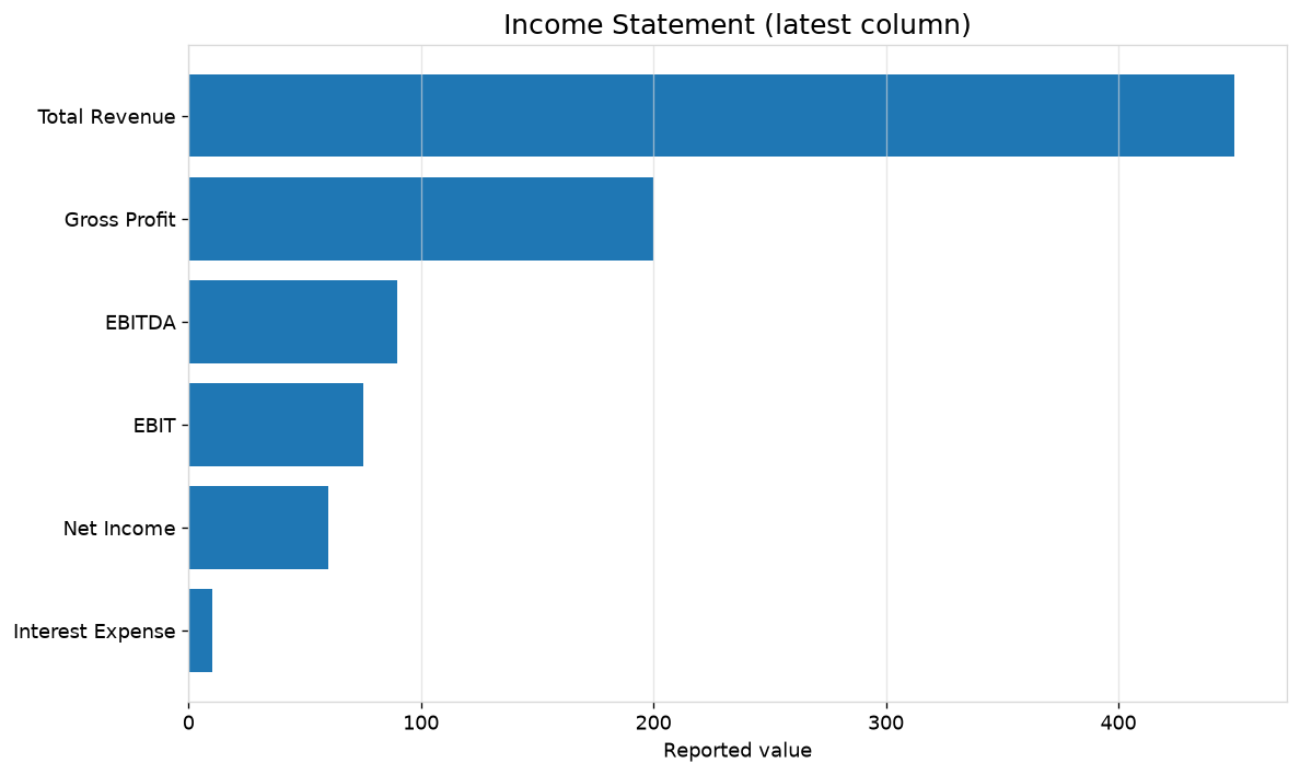
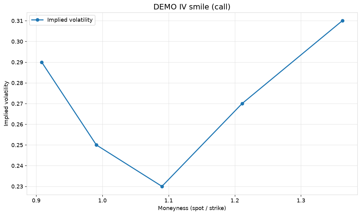
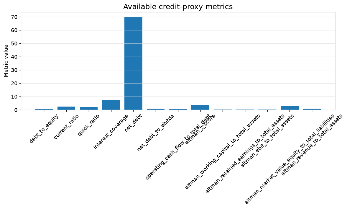
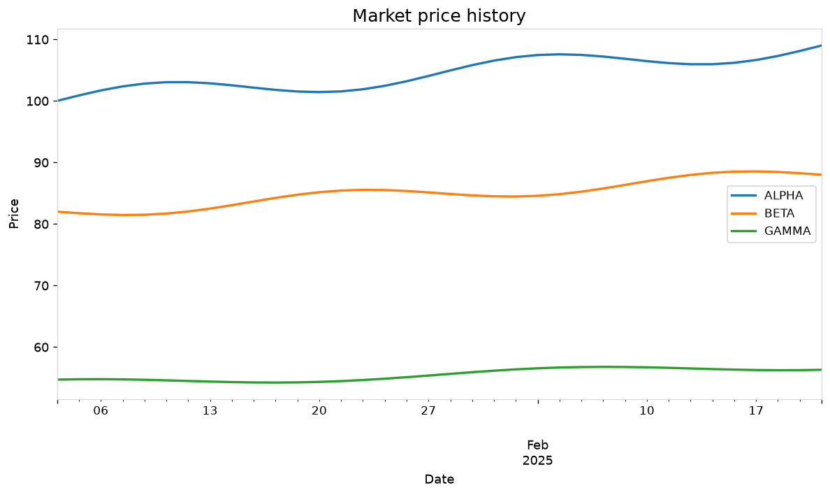
Price history, statement, and option-chain analytics charts, saved without an implicit show() call.

try:
    figures = {
        "ticker_history": ticker.visualize(period="1mo"),
        "income_statement": ticker.financials.visualize(statement="income_statement"),
        "option_iv_smile": chain_analytics.visualize(chart="iv_smile", option_type="call"),
        "credit_metrics": assessment.visualize(chart="metrics"),
        "universe_history": universe.visualize(period="1mo"),
    }
    print(f"Created {len(figures)} figures: {list(figures)}")
except VisualizationError as exc:
    print(f"Visualization skipped (optional dependency missing): {exc}")

Created 5 figures: ['ticker_history', 'income_statement', 'option_iv_smile', 'credit_metrics', 'universe_history']

Takeaway

MarketTicker/MarketUniverse give you the same interface whether the underlying data is a deterministic fixture (as here) or a live provider — see notebook 07 — Live Market Data (Yahoo/yfinance) and 15 — SEC EDGAR/XBRL Fundamentals for real-data variants.