Scenario Analysis

AbaQuant treats scenario analysis as a first-class workflow across three domains, all following the same pattern:

base case -> scenario grid -> visual report

Sections:

1. Derivative spot–volatility scenario grid

2. Portfolio one-period asset-shock scenario

3. Credit debt/EBITDA multiplier scenario

4. Summary and figures

Setup

import abaquant
print(f"AbaQuant version: {abaquant.__version__}")

AbaQuant version: 1.0.0rc1

import pandas as pd

from abaquant.credit import (
    BalanceSheetInputs,
    CashFlowInputs,
    CreditAnalysisInputs,
    CreditHistoricalSeries,
    IncomeStatementInputs,
    MarketEquityObservation,
    PriorPeriodInputs,
    calculate_credit_proxy_metrics,
)
from abaquant.derivatives.models import BlackScholesMertonModel
from abaquant.portfolio import PortfolioAllocator
from abaquant.visualization import VisualizationError

1. Derivative spot–volatility scenario grid

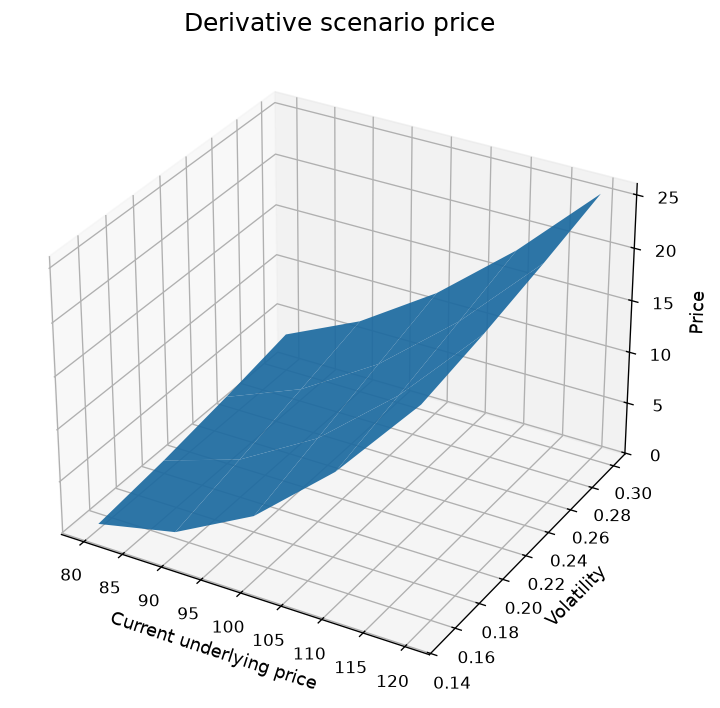
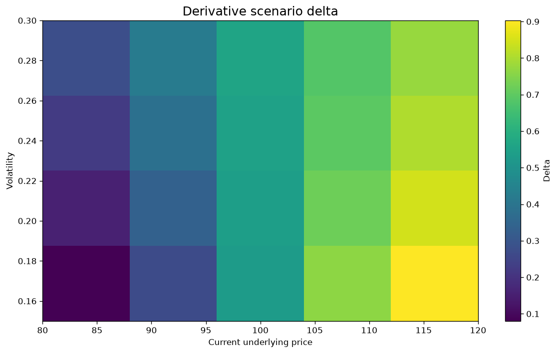
Evaluate a call option’s price and Greeks across a grid of spot prices and volatilities — useful for stress-testing a position ahead of an earnings announcement or macro event.

option_model = BlackScholesMertonModel(
    spot_price=100.0,
    strike_price=105.0,
    maturity_years=1.0,
    risk_free_rate=0.05,
    volatility=0.22,
)
derivative_grid = option_model.scenario_grid(
    spot_prices=[80.0, 90.0, 100.0, 110.0, 120.0],
    volatilities=[0.15, 0.20, 0.25, 0.30],
    option_type="call",
)
derivative_grid.data.head()

	option_type	spot_price	volatility	price	intrinsic_value	extrinsic_value	moneyness	forward_moneyness	break_even_price	delta	gamma	vega	theta	rho	vanna	volga	charm
0	call	80.0	0.15	0.410799	0.0	0.410799	0.761905	0.800968	105.410799	0.080076	0.012398	0.119019	-0.003267	0.059953	1.541847	173.249095	0.000453
1	call	80.0	0.20	1.199547	0.0	1.199547	0.761905	0.800968	106.199547	0.156327	0.014977	0.191705	-0.006801	0.113066	1.449372	117.070843	0.000561
2	call	80.0	0.25	2.284333	0.0	2.284333	0.761905	0.800968	107.284333	0.222811	0.014913	0.238601	-0.010300	0.155405	1.208196	73.722635	0.000577
3	call	80.0	0.30	3.556910	0.0	3.556910	0.761905	0.800968	108.556910	0.277669	0.013969	0.268206	-0.013578	0.186566	0.994349	46.915675	0.000562
4	call	90.0	0.15	2.048286	0.0	2.048286	0.857143	0.901090	107.048286	0.267847	0.024394	0.296387	-0.009112	0.220579	1.689051	94.148380	0.000648

2. Portfolio one-period asset-shock scenario

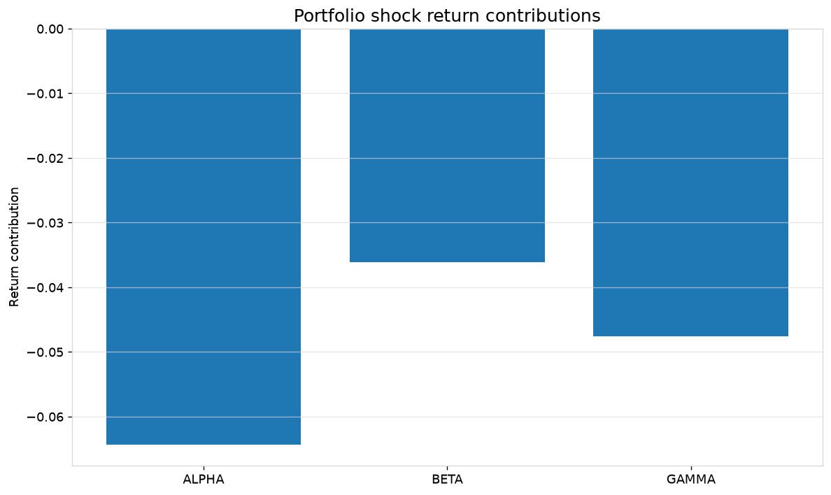
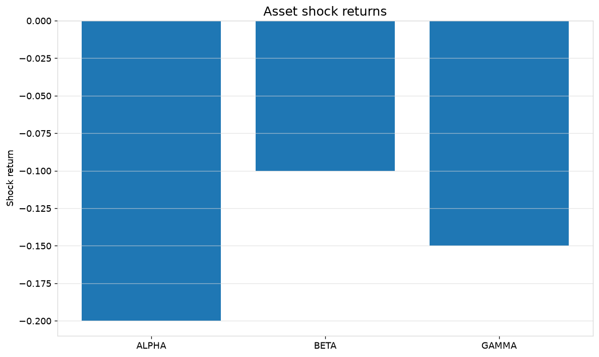
Apply an explicit percentage shock to each asset in a maximum-Sharpe allocation and see the resulting portfolio return and ending value.

returns = pd.DataFrame(
    {
        "ALPHA": [0.01, -0.002, 0.006, 0.004, 0.003],
        "BETA": [0.003, 0.005, -0.001, 0.002, 0.004],
        "GAMMA": [-0.002, 0.007, 0.004, 0.006, 0.001],
    }
)
allocator = PortfolioAllocator(returns, annual_risk_free_rate=0.02)
weights = allocator.mean_variance.maximum_sharpe()

portfolio_scenario = allocator.scenario_analysis(
    shocks={"ALPHA": -0.20, "BETA": -0.10, "GAMMA": -0.15},
    weights=weights,
    base_value=1_000_000.0,
)
print(f"Portfolio scenario return: {portfolio_scenario.portfolio_return:.4%}")
print(f"Ending value:              {portfolio_scenario.ending_value:,.2f}")

Portfolio scenario return: -14.8057%
Ending value:              851,943.07

3. Credit debt/EBITDA multiplier scenario

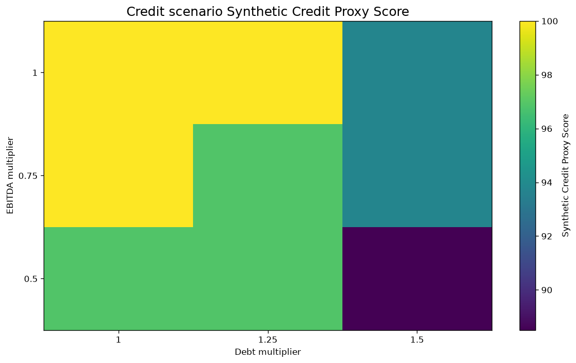
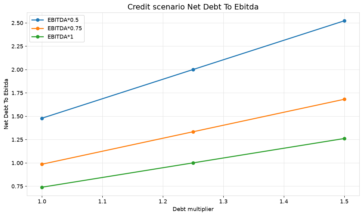
Stress a fundamentals-based credit-proxy assessment by scaling debt and EBITDA independently across a small grid, to see which input dominates the synthetic score.

assessment = calculate_credit_proxy_metrics(
    CreditAnalysisInputs(
        balance_sheet=BalanceSheetInputs(
            total_debt=120.0, total_equity=300.0, current_assets=180.0, inventory=20.0,
            current_liabilities=90.0, cash_and_cash_equivalents=35.0, total_assets=520.0,
            total_liabilities=220.0, retained_earnings=125.0, long_term_debt=105.0,
            shares_outstanding=100.0,
        ),
        income_statement=IncomeStatementInputs(
            revenue=700.0, gross_profit=310.0, ebit=90.0, ebitda=115.0,
            interest_expense=9.0, net_income=62.0,
        ),
        cash_flow_statement=CashFlowInputs(operating_cash_flow=78.0),
        prior_period=PriorPeriodInputs(
            total_assets=500.0, net_income=55.0, long_term_debt=112.0, current_assets=170.0,
            current_liabilities=95.0, shares_outstanding=100.0, gross_profit=290.0, revenue=660.0,
        ),
        market_equity=MarketEquityObservation(market_value_equity=950.0),
        historical_series=CreditHistoricalSeries(
            earnings_history=(46.0, 51.0, 55.0, 62.0),
            leverage_history=(0.54, 0.48, 0.43, 0.40),
        ),
    )
)
credit_grid = assessment.scenario_analysis(
    debt_multiplier=[1.0, 1.25, 1.50],
    ebitda_multiplier=[1.0, 0.75, 0.50],
)
credit_grid.data

	debt_multiplier	ebitda_multiplier	ebit_multiplier	interest_expense_multiplier	debt_to_equity	interest_coverage	net_debt_to_ebitda	altman_z_score	piotroski_f_score	synthetic_credit_proxy_score	synthetic_credit_proxy_band	available_score_weight
0	1.00	1.00	1.0	1.0	0.4	10.0	0.739130	5.052448	9	100.00	strong_balance_sheet_proxy	96.0
1	1.00	0.75	1.0	1.0	0.4	10.0	0.985507	5.052448	9	100.00	strong_balance_sheet_proxy	96.0
2	1.00	0.50	1.0	1.0	0.4	10.0	1.478261	5.052448	9	96.88	strong_balance_sheet_proxy	96.0
3	1.25	1.00	1.0	1.0	0.5	10.0	1.000000	5.052448	8	100.00	strong_balance_sheet_proxy	96.0
4	1.25	0.75	1.0	1.0	0.5	10.0	1.333333	5.052448	8	96.88	strong_balance_sheet_proxy	96.0
5	1.25	0.50	1.0	1.0	0.5	10.0	2.000000	5.052448	8	96.88	strong_balance_sheet_proxy	96.0
6	1.50	1.00	1.0	1.0	0.6	10.0	1.260870	5.052448	8	93.75	strong_balance_sheet_proxy	96.0
7	1.50	0.75	1.0	1.0	0.6	10.0	1.681159	5.052448	8	93.75	strong_balance_sheet_proxy	96.0
8	1.50	0.50	1.0	1.0	0.6	10.0	2.521739	5.052448	8	88.50	strong_balance_sheet_proxy	96.0

4. Summary and figures

Compact scalar highlights from all three scenario families, plus their visual reports.

summary = {
    "derivative_highest_call_price": float(derivative_grid.data["price"].max()),
    "derivative_lowest_delta": float(derivative_grid.data["delta"].min()),
    "portfolio_scenario_return": portfolio_scenario.portfolio_return,
    "portfolio_ending_value": portfolio_scenario.ending_value,
    "credit_lowest_proxy_score": float(credit_grid.data["synthetic_credit_proxy_score"].min()),
}
for key, value in summary.items():
    print(f"{key:34s}: {value}")

derivative_highest_call_price     : 25.522438407323904
derivative_lowest_delta           : 0.08007636126574669
portfolio_scenario_return         : -0.1480569262073188
portfolio_ending_value            : 851943.0737926812
credit_lowest_proxy_score         : 88.5

try:
    figures = {
        "derivative_price_surface": derivative_grid.visualize(metric="price", chart="surface"),
        "derivative_delta_heatmap": derivative_grid.visualize(metric="delta", chart="heatmap"),
        "portfolio_contributions": portfolio_scenario.visualize(chart="contributions"),
        "portfolio_shocks": portfolio_scenario.visualize(chart="shocks"),
        "credit_score_heatmap": credit_grid.visualize(
            metric="synthetic_credit_proxy_score", chart="heatmap"
        ),
        "credit_net_debt_curves": credit_grid.visualize(
            metric="net_debt_to_ebitda", chart="curves"
        ),
    }
    print(f"Created {len(figures)} scenario figures: {list(figures)}")
except VisualizationError as exc:
    print(f"Visualization skipped (optional dependency missing): {exc}")

Created 6 scenario figures: ['derivative_price_surface', 'derivative_delta_heatmap', 'portfolio_contributions', 'portfolio_shocks', 'credit_score_heatmap', 'credit_net_debt_curves']

Takeaway

Scenario grids give you a structured way to ask “what if” across derivatives, portfolios, and credit — without hand-rolling nested loops. Every result object exposes .data (a tidy DataFrame) plus .visualize() for a quick heatmap, surface, or curve chart.